Updating some U.S. House graphics

Now seems like a good time to remake some graphics I use often. All the underlying data are from Voteview.

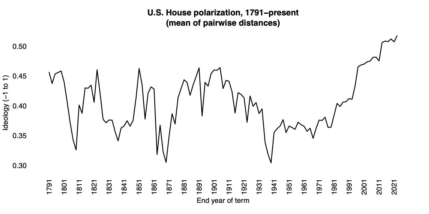
Below is a party-blind measure of polarization in the U.S. House, from the beginning of that chamber through Wednesday of last week. The party-blind measure is the mean of all pairwise distances. (I once calculated it here for states and first came across it here.) This lets us go back to before the major parties were Republicans and Democrats. It also does not force us to make arbitrary decisions about handling minor parties, independents, and others with less common ways of affiliating/identifying.

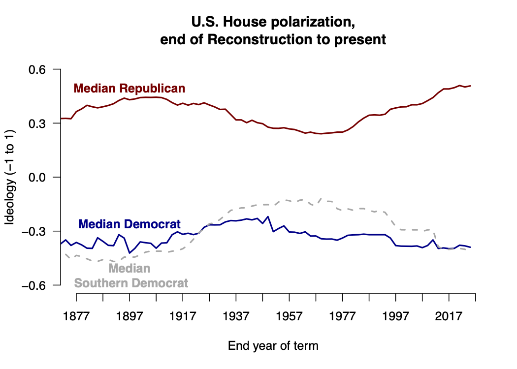
Below is the more familiar measure: distance between the median members of the major parties, back to the end of Reconstruction. This plot includes the median Southern Democrat (conventionally the 11 Confederate states plus Kentucky and Oklahoma).

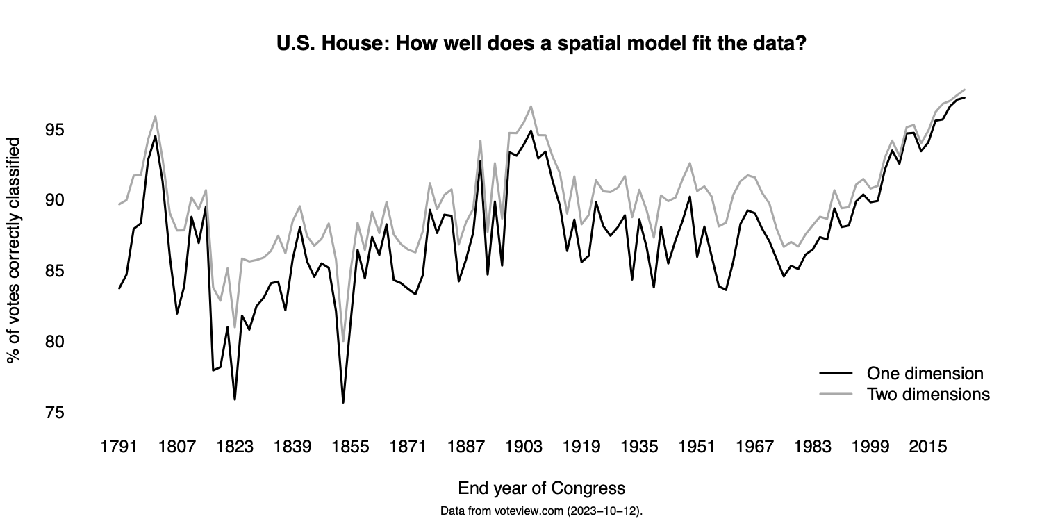
The last two plots answer the question: “How well does an N-dimensional model fit the data?” I used the optimal classification algorithm to recover ideal points for each House. I did this one Congress at a time; see here and here for other options. The black line comes from one-dimensional models. The gray line comes from two-dimensional models. The first plot gives the percentage of votes correctly classified, by Congress.

The second plot gives the aggregate proportional reduction in error.

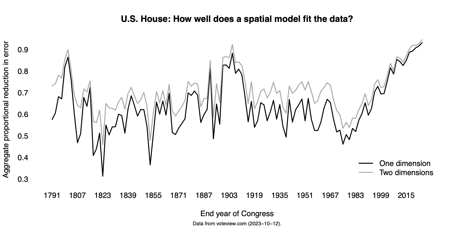
Here is a CSV of the fit measures above. The first two columns are for the one-dimensional models. The next two are for two dimensions.